Convolution related query

[23f3000345]

The explanation given for convolution was better than my signal and systems class, but there is only one example given based on this, what if the PDF vector’s length is less than kernel’s length and these vector’s are just 1d what happens in the higher dimension…

Also one more query related with example 2.10, what is the kernel vector and the PDF vector here in the example, it is not specified just the result of the convolution is given

Thanks in advance

[albertoezquerro]

Hello @23f3000345 ,

Hahaha! We’re happy you liked our convolution explanation! Let’s break down your questions step by step:

What if the PDF vector’s length is less than the kernel’s length (1D case)?

In traditional convolution, especially as done in signal processing or numerical simulation (like in the Bayes filter), the kernel is typically smaller than or equal to the input vector (PDF).

If the kernel is larger than the PDF vector, then you can’t fully slide the kernel over the input (it will hang off the edges). In this case, one of two things usually happens:

Option 1: Padding (most common)

• You pad the input with zeros (or other values) so that the kernel can fully slide across it.
• This is called zero-padding, and it allows the convolution to be computed without shrinking the result too much.
• For instance:
  • input = [1, 2]
  • kernel = [3, 1, 3]
  • You can pad input to: [0, 1, 2, 0]
  • Then perform convolution as usual.

Option 2: Output is undefined or skipped

• In very strict formulations, if the kernel doesn’t fit the input, the convolution may just return an empty array or error, depending on how it’s implemented.

---

What happens in higher dimensions?

In higher dimensions (2D, 3D, etc.), like in images or robot maps, convolution works very similarly, just extended across more axes.

For example, in 2D convolution (like for image filters):

• The PDF might be a 2D grid (e.g. a map of position beliefs).
• The kernel could be a 2D Gaussian (movement noise model).
• The kernel “slides” over the 2D belief grid, and at each position, performs elementwise multiplication and sum, just like in 1D.

If the kernel is larger than the input in 2D:

• Same options apply: you usually pad the input grid, or you restrict the valid output region (called valid convolution vs same convolution in deep learning terminology).

---

About Example 2.10:

You can get more info by checking the bayes_filter.py script in /home/user/catkin_ws/src/kalman_filters_files/bayes_tutorials/scripts. In this case:

PDF vector → belief

• Represents the robot’s current belief about its position.
• Initialized as:

belief = [0.1] * 10

Kernel vector → kernel

• Represents the motion noise model (i.e. how uncertain movement is).
• Initialized as:

kernel = [0.1, 0.8, 0.1]

In the predict_step(belief, offset, kernel) function:

• The belief is convolved with the kernel after shifting by offset, modeling noisy motion.

---

Hope this helps!

[23f3000345]

I got my answer but here one more thing I feel difficult to digest in the example given for convolution,

input = [1,0,2,3,0,1,1] and kernel = [3,1,3], convolution was applied quite simply meaning you start from input[0]*kernel[0] + input[1]*kernel[1] + input[2]*kernel[2] which gives the output[0] and you slide the kernel one by one and obtain the respective output indices but in the predict_step function there is one width variable which determines from where the kernel starts like it starts from kernel[0]*input[10]+kernel[1]*input[9] = output[0] and then kernel[0]*input[0]+kernel[1]*input[10] = output[1] and so on, and it feels quite confusing like you cannot I cannot intutively guess from where the multiplication is starting and I need to mug up that part of width…
Can you explain this in some intutive way? @albertoezquerro

[23f3000345]

[23f3000345]

@albertoezquerro Sir ??

[albertoezquerro]

Hello @23f3000345 ,

Let me try to explain everything in a more intuitive way

Simple Convolution

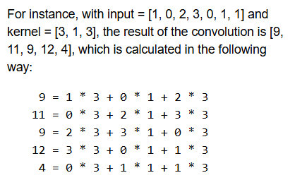
So from the image you shared, the basic convolution is done like this:

kernel = [3, 1, 3]
input  = [1, 0, 2, 3, 0, 1, 1]
output = [9, 11, 9, 12, 4]

Which is:

output[0] = 1*3 + 0*1 + 2*3
output[1] = 0*3 + 2*1 + 3*3
...

That’s standard convolution, where:

• Kernel is applied left-to-right
• We slide it over input
• We use padding (with 0s) so that we can apply it even at the edges

Now, the *"start at kernel[0]input[10]" kind of behavior feels strange because it’s not this “standard” form. That’s circular convolution, with a reversed kernel.

---

Now Let’s Decode This Formula:

index = (i + (width - k) - offset) % N

Let’s understand each piece step by step.

i: output index

You’re computing output[i].

k: position in kernel (e.g., k=0 is the first kernel element)

width - k: This flips the kernel

Think of it like we want to align the end of the kernel with the current position i.

If kernel = [a, b, c], then flipped it becomes [c, b, a].

offset: Where to center the kernel

This helps you decide whether kernel[1] aligns with input[i], or maybe kernel[0] or kernel[2] does.

If offset = width // 2, the kernel is centered.
If offset = 0, it’s causal (kernel is fully behind the current index).

% N: Wraps the input (makes it circular)

---

So What Does It All Mean?

Think of it like this:

“To compute output[i], flip the kernel, shift it back by offset, and apply it to the input values wrapping around the array.”

So if:

• width = 3 (kernel has 3 elements)
• offset = 1 → center the kernel at i
• Then:

index = (i + (3 - k) - 1) % N
       = (i + 2 - k) % N

So for each k = 0, 1, 2, you’re grabbing:

• input[i + 2 - 0] → for k=0 → input ahead of i
• input[i + 2 - 1] → for k=1 → input at i+1
• input[i + 2 - 2] → for k=2 → input at i

So this setup is applying the reversed kernel, centered at i.

---

---

Hope this helps clarify things a little bit!